Motivation

The greatest value of a picture is when it forces us to notice what we never expected to see. ~ John Tukey

Yesterday, Matt Harrison shared his recreation of Our World In Data’s graphical trend of Kyoto’s Cherry trees blossoming, encouraging other data scientists and analysts to try it out to enhance their visualization skills.

In my humble opinion, replicating others’ work is an effective learning strategy. As a result, this tutorial aims to recreate an intriguing visual by Our World in Data. My objective is to practice and improve my visualization skills and help those new to R programming and the ggplot2 library (I could have done this with the pandas and seaborn libraries; however, I am more comfortable with the ggplot2).

Getting Started

Loading the Required Libraries

In this tutorial, I will load two packages - tidyverse and ggtext. Later, in the visualization section, I will use the ggthemes package and call it directly since I need a single theme to enhance my plot.

# Libraries ------
library(tidyverse)
library(ggtext)

Data Wrangling and Visualization

Cleaning and Transforming data

Importing the Dataset

In this section, I will use the link from Matt Harrison’s post to load the Kyoto Full Flower 7 dataset. After loading the data, I will write a function to clean and transform it and demonstrate how to write a function in R.

# Load the dataset
cherry_raw <-
  readxl::read_excel(
    "KyotoFullFlower7.xls",
    skip = 25
  ) |>
  janitor::clean_names() |>
  select(
    year = ad,
    flowering_day_of_year = full_flowering_date_doy,
    flowering_month = full_flowering_date
  ) |>
  mutate(
    date = str_c(year,
      str_sub(flowering_month, 1, 1),
      str_sub(flowering_month, 2, 3),
      sep = "-"
    )
  ) |>
  filter(!is.na(date)) |>
  mutate(
    rolling_day_of_year = slider::slide_dbl(
      flowering_day_of_year,
      mean,
      .before = 20,
      .complete = TRUE
    )
  )

In the code snippet above, I used the read_excel() function from the readxl package to read the KyotoFullFlower7.xls dataset. I then skipped the first 25 rows with the skip() argument, converted column names to snakecase using the clean_names() function from the janitor package, and selected and renamed the columns of interest with the select() function from the dplyr package.

After that, I created a new column named “date” by combining the year with the month and day portions of the “flowering_month” column. I used the str_c() and str_sub() functions from the stringr package for this purpose. The new column values were separated by a hyphen (“-”) to look like “year-month-day,” for example, “815-4-15”. Then, I removed missing or NA values from the new date column using the filter() function from the dplyr package.

Finally, I calculated the mean “rolling_day_of_year” with the slide_dbl() function from the slider package. I used a 20-year window and the values were calculated from the flowering_day_of_year.

Writing a Function

# Define a function for cleaning and transforming dataset
tweak_cherry_trees_data <- function(data,
                                    window,
                                    cols) {
  data |>
    janitor::clean_names() |>
    select({{ cols }}) |>
    mutate(
      date = str_c(year,
        str_sub(flowering_month, 1, 1),
        str_sub(flowering_month, 2, 3),
        sep = "-"
      )
    ) |>
    filter(!is.na(date)) |>
    mutate(
      rolling_day_of_year = slider::slide_dbl(
        flowering_day_of_year,
        mean,
        .before = {{ window }},
        .complete = TRUE
      )
    )
}

In the above code snippet, I wrote a data cleaning and transformation function using the code in the preceding section. I will not dive deep into the mechanics of function writing in R in this section; those interested can read more about R function writing here.

Testing the Function

# Let's test our new function
cherry_trees_raw <-
  readxl::read_excel(
    "KyotoFullFlower7.xls",
    skip = 25
  )

# Clean and transform the data
cherry_trees_data_tbl <-
  tweak_cherry_trees_data(
    cherry_trees_raw,
    cols = c(
      year = ad,
      flowering_day_of_year = full_flowering_date_doy,
      flowering_month = full_flowering_date
    ),
    window = 20
  )

My new function worked well, and I can now use it to update my analysis of the cherry trees blossoming in Kyoto whenever necessary.

Plotting Cherry Trees Data

# Plot cherry trees data ------
cherry_trees_data_tbl |>
  ggplot(aes(year, flowering_day_of_year)) +
  geom_point(na.rm = TRUE, size = 0.8) +
  geom_line(
    aes(y = rolling_day_of_year),
    na.rm = TRUE,
    linewidth = 1.2,
    color = "#5e2ce8"
  ) +
  annotate(
    "text",
    x = 1990,
    y = 90,
    label = "20-Year\n Average",
    color = "#5e2ce8",
    size = 8,
    na.rm = TRUE
  ) +
  scale_x_continuous(
    limits = c(812, 2015),
    breaks = c(812, 1000, 1200, 1400, 1600, 1800, 2023)
  ) +
  scale_y_continuous(
    limits = c(70, 120),
    labels = c(
      "March 11", "March 21", "March 31",
      "April 10", "April 20", "April 30"
    )
  ) +
  ggthemes::theme_wsj() +
  labs(
    title = "Cherry trees have been blossoming earlier due to warmer spring temperatures",
    subtitle = "Date of peak cherry tree (***Prunus jamasakura***) in Kyoto, Japan",
    caption = "**Data Source: Yasuk Aono (2021:2024)**<br>**Note:** The <span style='color: #5e2ce8'>20-year average</span> is calculated when there are at least five years with data in the <span style='color: #5e2ce8'>20-year window</span>. The dates are off by one day on the years.<br><br>
        OurWorldInData.org/biodiversity|CC BY
        "
  ) +
  theme(
    plot.title = element_textbox_simple(
      size = 30,
      margin = margin(t = 15, r = 0, b = 5, l = 0),
      lineheight = 1.2,
      linewidth = 0.3
    ),
    plot.title.position = "plot",
    plot.subtitle = element_textbox_simple(
      size = 20,
      hjust = 0,
      margin = margin(t = 15, r = 0, b = 15, l = 0),
      lineheight = 1.2,
      linewidth = 0.1
    ),
    axis.text = element_textbox(
        size = 13, 
        color = "darkgray"
    ),
    plot.caption = element_textbox_simple(
      size = 20,
      margin = margin(t = 15, r = 0, b = 10, l = 0),
      lineheight = 1.2,
      linewidth = 0.1
    ),
    axis.line = element_line(color = "darkgray"),
    axis.ticks = element_line(color = "darkgray"),
    plot.caption.position = "plot",
    plot.margin = margin(15, 15, 15, 15)
  )

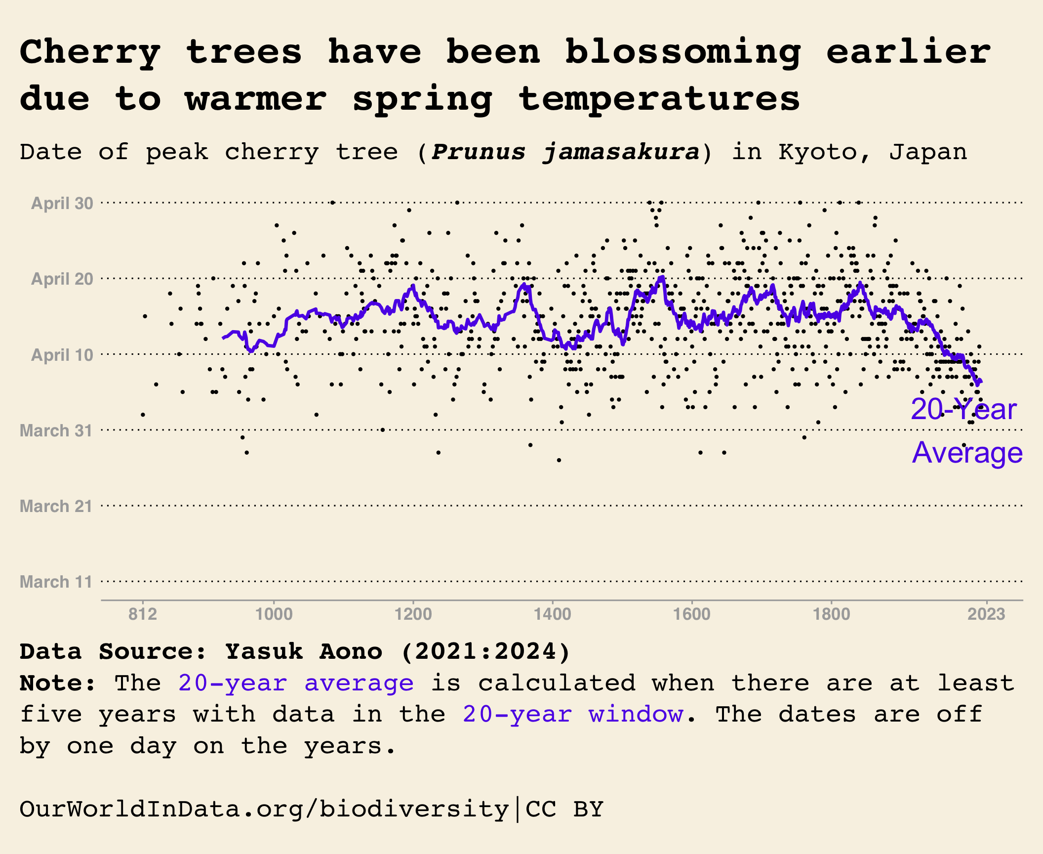
I created a scatter plot with the x-axis representing the year and the y-axis representing the flowering day of the year. To do this, I used the geom_point() function and set the point size to 0.8. I also plotted a line graph of the 20-year rolling average using the geom_line() function. I made the line thicker and colored it in purplish color. I added a text label “20-year average” using the annotate() function and modified its location, color, and size as shown above.

To make the plot resemble that of Our World In Data graph, I controlled the axes by setting the limits, breaks, and labels accordingly. I used Matt Harrison’s code along with the original graph as a guide. Additionally, I used the theme_wsj() function from the ggthemes package to mimic the original graph.

Finally, I polished the plot with the theme() function to make it look as much as possible like the original plot. I will not explain every argument here for the sake of time.

Final Thoughts

In this tutorial, I demonstrated how to load KyotoFullFlower7.xls, clean and transform it, write a function that automates the wrangling process, and visualize the cleaned data to replicate the original graph.
This simple recreation of the Our World In Data graphic has become a beautiful tutorial worthwhile for those interested in data visualization with the ggplot2 package.
My goal was to recreate the plot and help those new to R learn how to do the same thing.

Overall, this tutorial demonstrates how to recreate a visually informative plot showcasing the trend of cherry blossom flowering dates in Kyoto, Japan, with annotations and proper citation.
Please leave us a comment, share our tutorial, try it yourself, and share your work with me and the Data Science Community.

Acknowledgements

I would like to express my gratitude to Matt Harrison for introducing me to this excellent exercise and for being a constant source of inspiration. Additionally, I extend my thanks to Our World In Data for their valuable contributions and for making the data accessible to everyone for practice purposes.